

If you want to apply conditional formatting based on the value of another cell including text or number or date etc., then this can be achieved by creating a rule in conditional formatting using a custom formula.
Example of conditional formatting based on the value of another cell
In the example below, we want conditional formatting on cells with figures that fall below the yearly average.
Select the cells you want to format. You can select one column, several columns, or the entire table if you wish to apply your conditional format to rows.
Tip: If you want the conditional formatting rule to get applied to new data entries automatically, you can either:
- Convert a range of cells to a table (Go to the Excel Ribbon on the Insert tab > click Table). In this case, the conditional formatting will be automatically applied to all new rows.
- Select some empty rows below your data, say 100 blank rows.
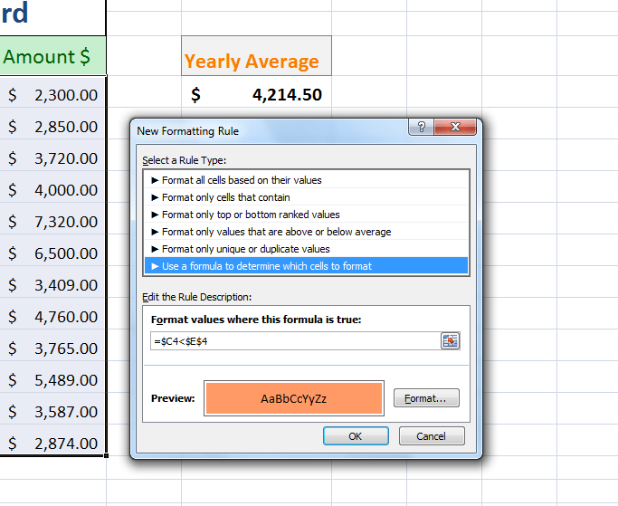
Select the data cells in B4:C15 range, click the Home tab of the Excel Ribbon and then select Conditional Formatting → New Rule.
This opens the New Formatting Rule dialog box. Click the “Use a Formula to Determine Which Cells to Format” option.
In the formula input box, enter the formula to compare your data range values (B4:C15) with the value in the comparison cell ($E$4).
Here, as you are only comparing the sales figures in column C with yearly average figure in cell $E$4, so you will fix the column by using $ sign with column name, and will keep the row number free or relative to evaluate each cell value in column C against value based on cell $E$4.
=$C4<$E$4
This formula will compare the sales figures in column C with yearly average value in cell $E$4, and will conditionally format the data rows in the selected range.
Then, click the Format button and select the option for formatting of font, border, and fill for your target cells. Click the OK button to confirm your changes and return to the New Formatting Rule dialog box. Again press OK button to confirm your formatting rule.
As you want to apply conditional formatting based on cell value of $E$4, so the above formula will evaluate the results in column C based on the value in $E$4 and conditional formatting will take effect where the formula will return TRUE.
Monthly sales data will be highlighted conditionally as per your chosen format if it is less than the yearly average figure in E4 as shown below.


Trying to apply conditional formatting to a block of cells based on content of one of those cells. I need to highlight w/ one of four colors. The colors are based on criteria within a large list of model numbers that contain letters and numbers. Each color would apply to a portion of those model numbers
Nice article! I have a spreadsheet that has coloured cells ( conditional formatting ).. There are 7 sites with 12 results per site, highlighted Red or Green in cell depending on how they are doing I want to rank each site across the 7 be the best wit the most green cells out of their 12 areas per site
I need to link the value of a drop down option to a COUNTIF function between tabs. Also, I need to use a conditional formatting function to give a pass/fail grade depending on the numbers generated from the previous functions. This is all between sheets in the same workbook.
I cannot figure this step out and need help please. Step 1: At this point, a smaller list of countries should be visible in the worksheet “Internet user and pop. Table”. Cross reference these countries with the list of tech ready countries in the “Tech Readiness 2016” and highlight in the “Internet user and pop. Table” worksheet the country or countries that are in both lists. You may choose any shade of orange as the highlighting color. Cross reference them using conditional formatting.
I am trying to form a list of duplicates in a large spreadsheet. I have already done conditional formatting to highlight duplicates in two columns but cannot extract the duplicates to a separate list.
I need to know how I can make this Google Sheet file an excel file while preserving all of its conditional formatting functions.
May I ask help on creating a conditional formatting? I would like to make 95% and above as green then orange for 80%-94% and red for 80% below.