

If you want to highlight cells based on a value as criteria, then you can use conditional formatting by using a built-in rule and a custom formula. This tutorial will show you how with several illustrated examples.
Use conditional highlighting to highlight cells less than or greater than a value
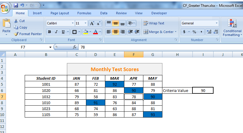
In the example below, you will set conditional formatting so that a cell:
-
- Turns dark Blue if it contains a value greater than 90
- Turns dark Blue if it contains a value greater than equal to 90.
Using the Built-in Rule
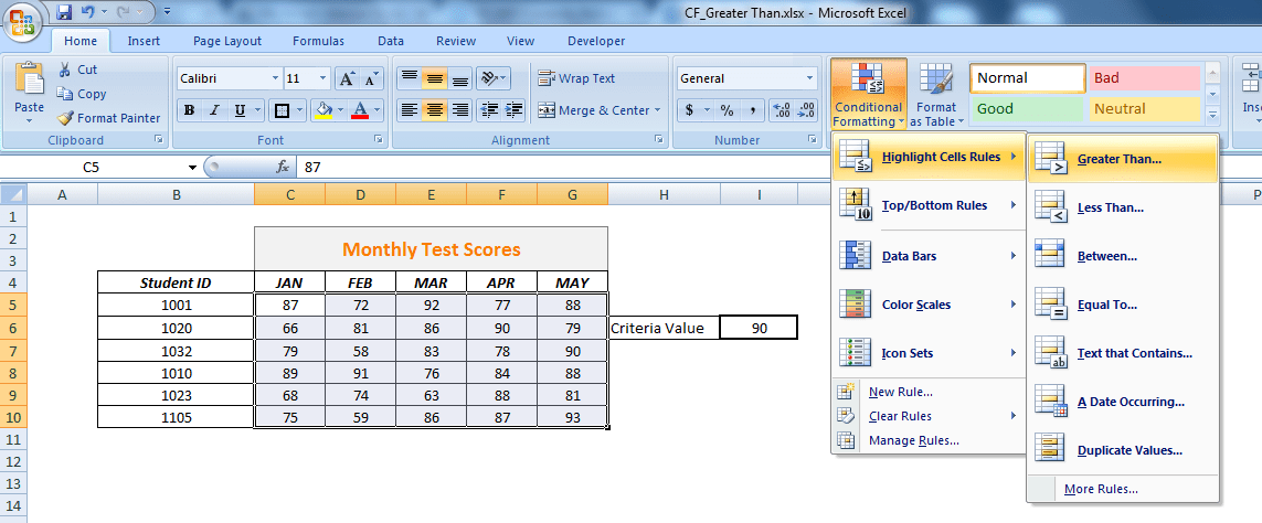
Select the range you want to format. In our case C5:G10 is selected. On the Excel Ribbon’s Home tab, click Conditional Formatting, to format the values greater than a specific one, select Highlight Cells Rules and then choose the option Greater Than.
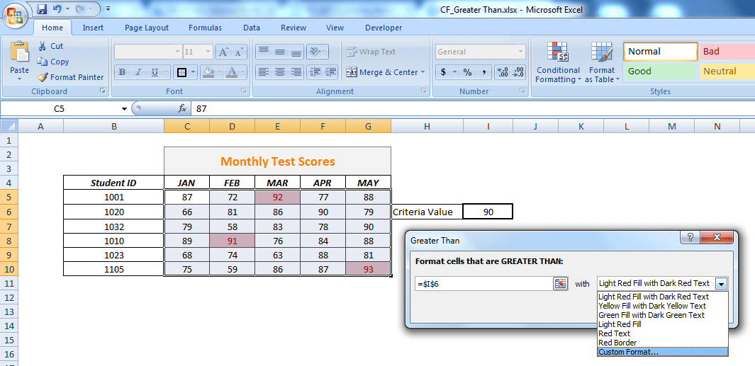
In the Greater Than window, you have to delete the value that appears in the box, and then select the cell reference, in this example $I$6, or input specific value that is the lowest limit for you.
To drop down the list for formats click Custom Format, click the Fill tab, and click on the blue dark fill color that you want.
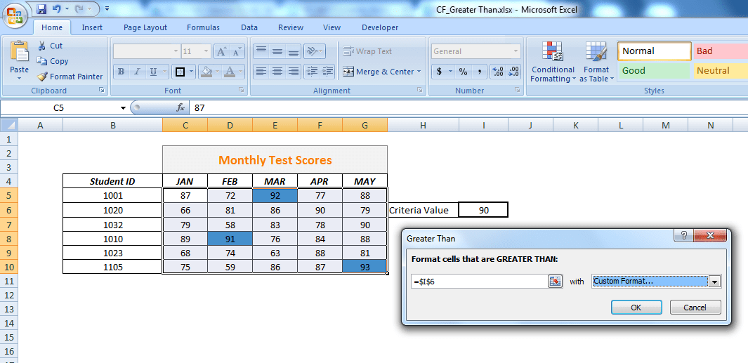
To close the Format cells window click Ok, the cells with values greater than 90 would be colored dark blue as you choose the color format. Again press OK
Using customer Formula Rule
You can conditionally highlight the cells which are greater than or equal to set a value using customer-formula rule.
Select the cells to be formatted. In this example, cells C5:G10 is selected, From the Home tab, click the Conditional Formatting selection. Click on “New Rule” and click on “Use a formula to determine….” and enter following formula in Edit Rule Description window. Choose Format > Fill > Dark Blue color to preview and press OK.
=C5>=$I$6
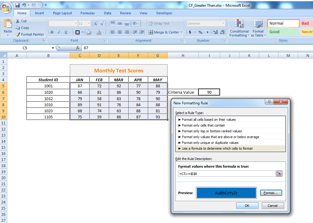
This formula will check all the active cells in the selected range and will test each cell value against the set value in cell $I$6. All those cells will be highlighted which are greater than equal to a set value of 90.
Need some additional help with Conditional Formatting or have other questions about Excel? Connect with a live Excel expert here for some 1 on 1 help. Your first session is always free.


It is helpful! Thanks!