Learn How to Apply Conditional Formatting in a Pivot Table

A pivot table in Excel is an excellent tool for analyzing data. It helps you to aggregate, summarize, find insights, and present a large amount of data in just a few clicks. You can create and change pivot tables very quickly. Conditional formatting is an excellent way to visualize data in Excel. It enables you to highlight cells with a format of your choice, depending on the cell’s value. In this tutorial, we will see how to combine conditional formatting with pivot tables.

Conditional Formatting in a Pivot Table

Conditional formatting in pivot tables allows us to visualize the pivot table data efficiently. In the following example, you have the beverage sales data of eleven items for the 2nd quarter of the year.

To create the Pivot Table and apply conditional formatting, you need to perform the following steps:

1. Click anywhere in the data.
2. Go to Insert > Recommended PivotTables. Scroll down and select the one that says Sum of Sales by Items and Month.

3. Click OK.

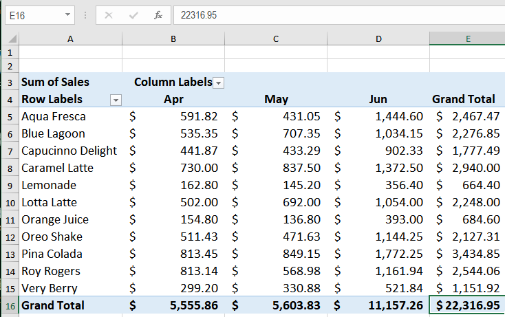
You will have the pivot table with the Sales for the Items for each Month.

Conditional Formatting in Pivot Table Based on Built-in Presets

To apply conditional formatting in a pivot table, you need to select a group of cells and apply a conditional formatting rule. However, you need to set the correct option from the pivot tables formatting options immediately after applying the conditional format rule. This would make sure the formatting works even after you change the data for the pivot table.

In the previous example, if you wanted to highlight sales for items that are greater than $520.00, you need to follow these steps:

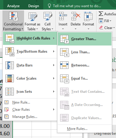
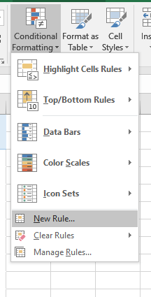
1. Select cells B5:D15 on the pivot table.
2. Go to Home > Conditional Formatting > Highlight Cell Rules > Greater than.

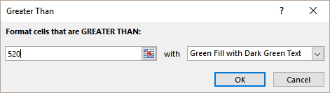
3. In the Format cells that are Greater than box type 520. Set the fill as Green fill with Dark Green text.

4. Click OK.

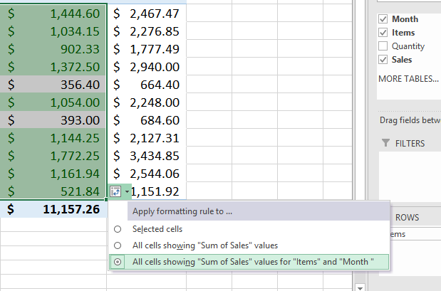
This will highlight the values greater than $520.00 with a green fill and dark green text. However, this will only set the conditional format to the fixed range from B5:D15. Each time you update the pivot table data, the conditional format would not be applied to the new range.

To fix this, immediately after you apply the conditional format rule, click on the Formatting Options icon on the bottom right. Select All cells showing “Sum of Sales” values for “Items” and “Month.” This will make sure the formatting is intact even if the data is updated.

Conditional Formatting in Pivot Table based on Formulas

You can assign Excel’s preset conditional formatting rules to your data. However, you can also add custom rules to format data. In this example, you will use the sales for the 3rd quarter and apply conditional formatting based on a formula. You now have the sales of items for the 3rd quarter. From this, we have the pivot table Sum of Sales by Items and Month.

Let’s say you want to find out the months where the items had bigger sales than the previous month. To find this out, you need to:

1. Select cells C5:D15(We leave column B out of the selection because it is the first month of the quarter and does not have any preceding value).
2. Go to Home > Conditional Formatting > New Rule.
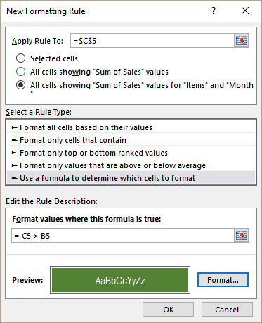
3. Under Select a Rule Type click Use a formula to determine which cells to format. In the Format values where the formula is true box assign the formula = C5 > B5.
4. To keep the conditional formatting working even if the pivot table is updated check the All cells showing “Sum of Sales” values for “Items” and “Month” on the top.

5. Click on Format. Select the Fill color as Green and Font color as White. Click OK to confirm the format.
6. Click OK to apply the formatting to the cells.

Pivot tables are a great way to summarize and aggregate data to model and present it. You can now visualize and report data in the blink of an eye, all thanks to pivot tables. Dashboards and other features have made gaining insights very simple using pivot tables.

Conditional Formatting is another fantastic tool in Excel. Shipping with essential presets, you can also add your custom made rules to conditional formats. In this tutorial, we saw how you could use conditional formatting within the pivot table to make your data more presentable in an effective and efficient way.

There are many interesting features of Pivot table and conditional formatting that could help you gain insights into your data. If you want to save hours of researching and frustration and get to the solution quickly, try our Excel Live Chat service! Our Excel experts are available 24/7 to answer any Excel question you have on the spot. The first question is free.