How to Create Calculated Fields in a Pivot Table

Pivot Tables are the most powerful tools in Excel to analyze a big set of data in a flexible way. You can quickly and easily build a complicated report to summarize your findings from your dataset. You can even customize the functionality of your pivot table with a Calculated Field.

Create calculated fields in a pivot table

What is a Calculated Field?

The Calculated Field is a built-in feature of the Pivot Table to further enhance its functionality and do calculations on your data to get the desired results by creating your own formula. You can use Calculated Fields to add a new field within your Pivot Table to do and display the calculations based on values of fields in your dataset.

In other words, by using Calculated Fields, you can easily add/subtract the values of 2 fields; make calculations based on some conditions/criteria in a formula by using data of a field(s) to show the results in a newly added field within the Pivot Table. We can make a variety of calculations in Calculated Fields, like dividing, subtracting, multiplying two or more fields, sum divided by count of the field, count, average, weighted average, even IF statements to make calculations based on criteria.

Using the Calculated Field in a Pivot Table

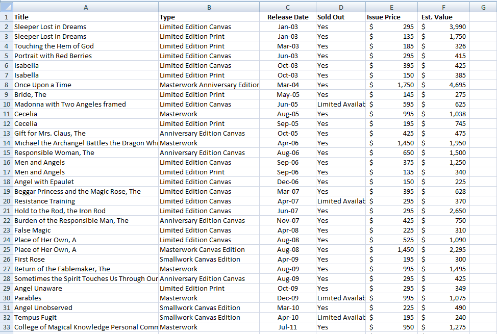
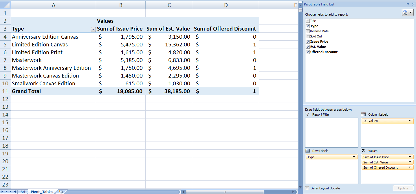
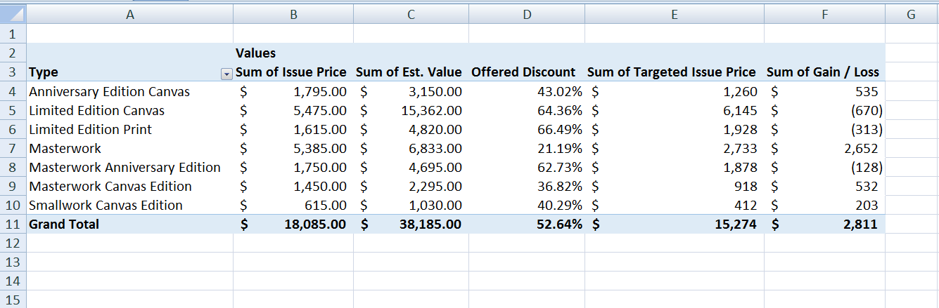
In this tutorial, we will use a data set of Art Gallery Exhibition as an example. Let’s imagine you are an Art Gallery manager who wants to compare the data set of Estimated Value and Issue Price (Actual Sold Price) for each item under a certain defined category.

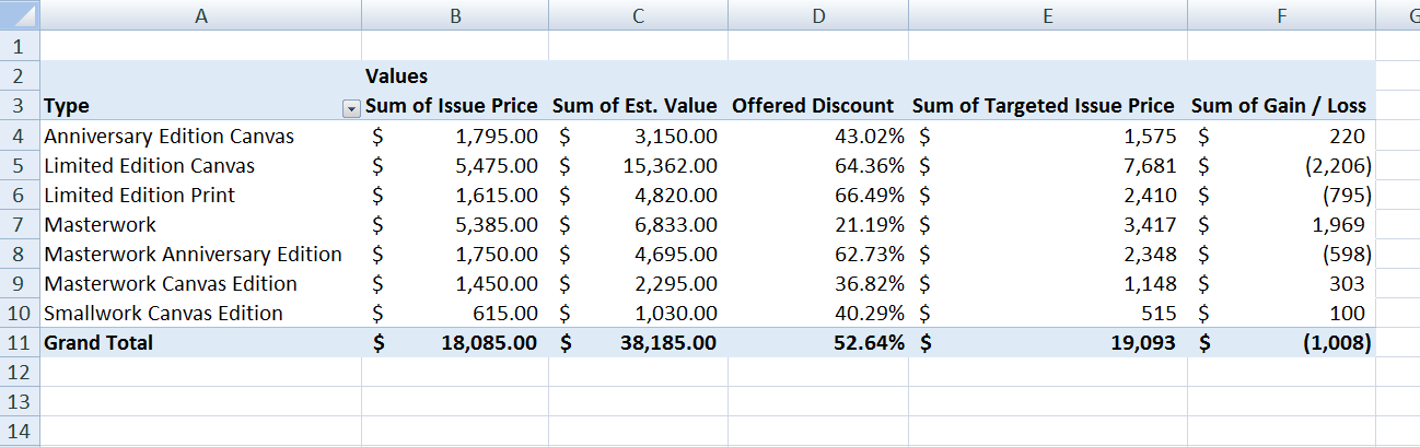
By using a Pivot Table, you can calculate the sum of Est. values, and the sum of Issue prices for all the items based on their categories. In addition to this, you can see how much of a discount you have offered for each category as a result of Est. Value and Issue Price difference. And you can also see how much Gain/Loss you have made in the context of a targeted flat discount rate, say 50%.

For these other requirements, you will be working with Calculated Fields in your Pivot Table, named “Offered Discount,” “Targeted Issue Price” and “Gain/Loss.”

Here, you will learn how to create, change and add/subtract 2 Fields in Pivot Table using this a data set of Art Gallery Exhibition.

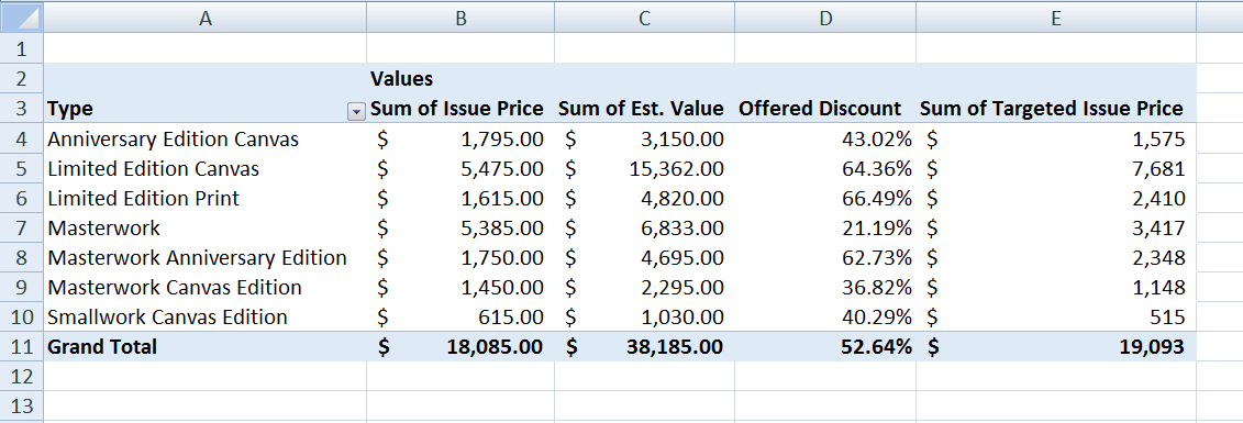
Let’s have a look at the below Pivot Table where you need to do basic calculations to sum Issue Price and Est. Value for each Type of defined category.

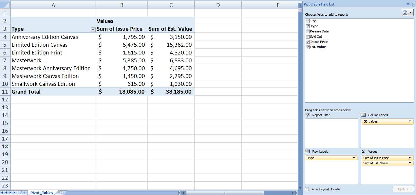
Now, we need to add or create the above-mentioned Calculated Fields into the Pivot Table. This use values of these fields, as shown in the above image, in the formula to make calculations.

How to add/create Calculated Fields in a Pivot Table

The Calculated Fields are added, one by one in the following steps.

1. Click any cell inside the pivot table.

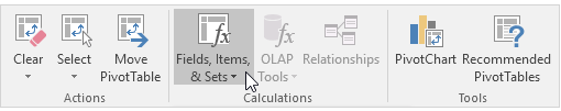
2. On the Analyze tab, in the Calculations group, click Fields, Items & Sets.
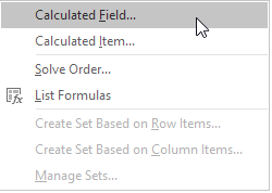
3. Click Calculated Field.

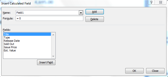
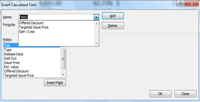
   The Insert Calculated Field dialog box appears.

4. Enter Name of Calculated Field
5. Type the formula
6. Click Add.

   Note: use the Insert Field button to quickly insert fields when you type a formula. To delete a calculated field, select the field and click delete (under Add).

7. Click OK. Excel automatically adds the Calculated Field to the Values area of the Pivot Table.

Repeat these steps to add all Calculated Fields as per following names and their respective formulas to make calculations.

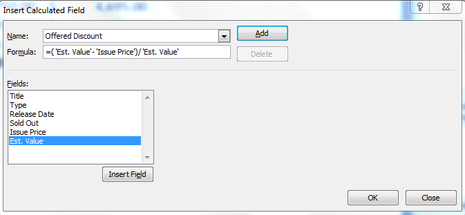
1. Offered Discount. This field will use the values of following Pivot Table fields in the below-mentioned formula. (See image)
   Formula: = (‘Est. Value’ – ‘Issue Price’) / ‘Est. Value’

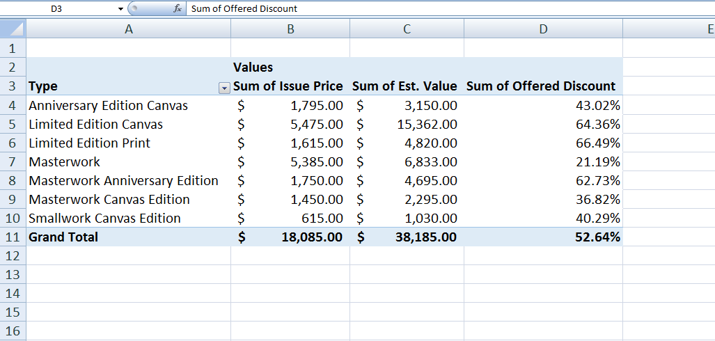
   Excel will automatically add this field in the Values area of the Pivot Table, but it will show as “Sum of Offered Discount”. We need to change the format for this field as Percentage and edit its name to show as “Offer Discount “ (See image).

   We need to do following to make changes in Format and Name of Field as per the requirement.

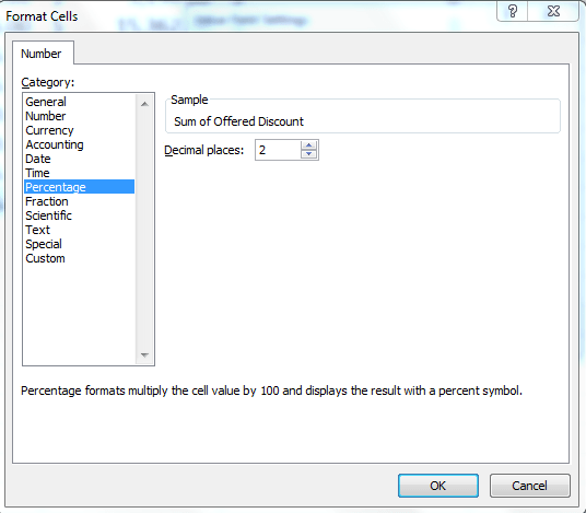
   To change its format from Sum of values to Percentage, we need to do following:

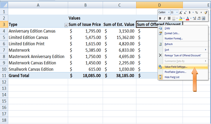
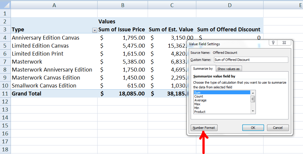
   Right-Click on the name of the Calculated Field and select “Value Field Settings…” (See image)

   Then click on “Number Format” button to select Percentage as format option and press OK. (See image)

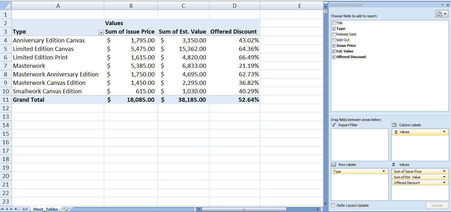
   Now, keep the cursor in this newly added Calculated Field and edit its name in the formula bar above, and press Enter. (See image)

   Following these steps, we will add the other two Calculated Fields below.

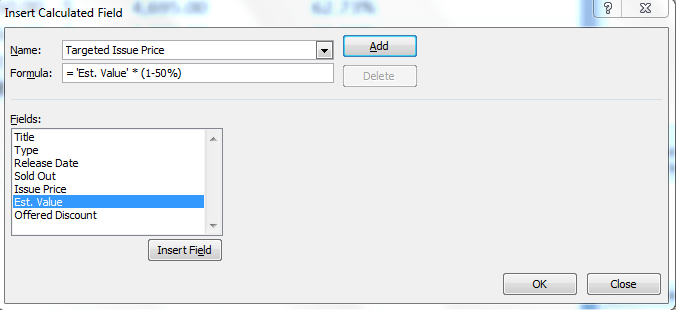
2. Targeted Issue Price. This field will use the values of following Pivot Table fields in the formula below. Formula: = ‘Est. Value’ * (1-50%)

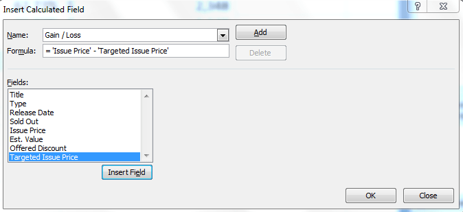
3. Gain/Loss. This field will use the values of following Pivot Table fields in the formula below.
   In this Calculated Field we will use two Fields to add/subtract to make calculations for this 3rd Calculated Field; one Pivot Table field and one Calculated Field as given below.Formula: = ‘Issue Price’ – ‘Targeted Issue Price’

   You can see all three Calculated Fields have been added within the Pivot Table using formulas to easily make calculations using existing fields.

How to modify Calculated Fields within a Pivot Table

Once you have created Calculated Fields, you can easily modify any of them. Just select the name of the Calculated Field from the drop-down list button of the Name section. Then, edit or modify the formula and click on modify button. See below pictures.

Here, you can see we have edited or modified the formula by changing the percentage from 50% to 60%.

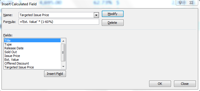
Here, you can see, by modifying the formula in one Calculated Field, all the relevant calculations have been updated in Pivot Table.

The calculated fields feature in the Pivot table is a powerful tool to perform quick calculations. There are many other Pivot table options that you can modify to achieve your calculation objectives.

If you haven’t found your answer in this article, try connecting to our experts using the link to the right. You will be connected to a qualified Excel expert in a few seconds, and they will solve your problem on the spot in a live, 1:1 chat session.