

Create a distinct list of items using Pivot Table
You can use the pivot table to create a distinct list of items. In the following example, you have the beverage sales data of eleven items for the 3rd quarter of the year.

There are 133 entries in this data each containing the Month, Items, Quantity and Sales for the 3rd quarter of the year. To create a distinct list based on quantity and sales for Items using pivot table you need to follow the next steps:
- Click anywhere in the data.
- Go to Insert > PivotTable.
- Check if the range covers the data. Check New Worksheet. Click OK.
![]()
- Look at the resulting pivot table worksheet, from the PivotTable Fields Menu on the right. You would need to set the fields into the appropriate labels.
- Set Items to the Row Labels. Quantity and Sales to the Value Labels.
![]()
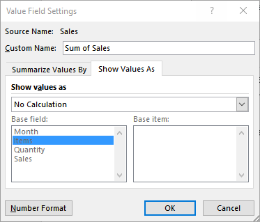
- Right-click anywhere in the Sum of Sales column in the pivot table. Select Value Field Settings > Show Values As > Number Format > Accounting. Click OK twice.
![]()


This will create a pivot table containing quantity and sales for a distinct list of Items for our data set.
Using Pivot Table for summation of one column and maximum of another. In this section, you will use the pivot table to sum one column based on distinct values and find the maximum of another based on the same values.
You will use the SoftTech IT project management data set for this example. The data includes the spending record and estimation for different tasks.
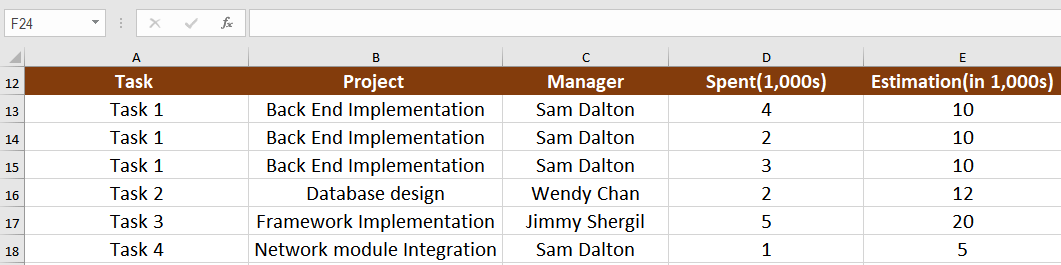
There are 6 entries each having the fields Task, Project, Manager, Spent(1,000s) and Estimation(1,000s).
In order to calculate the sum of the amount spent based on Task and compare it with the Estimation for that Task, you need to perform the following steps:
- Click anywhere in the data.
- Go to Insert > PivotTable.
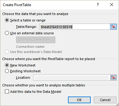
- Check if the range covers the data. Check New Worksheet. Click OK.
![]()
- View the resulting pivot table worksheet, from the PivotTable Fields Menu on the right. You would need to set the fields into the appropriate labels.
- Set Project to Filter Labels, Estimation (1,000s) to Column Labels, Spent (1,000s) to Value Labels, Task, and Manager to Row Labels.
![]()
- Go to Pivot Tables Tools > Design, click on Report Layout, and select “Show in Tabular Form”.
![]()
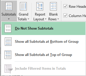
- Click on Subtotals and select “Do Not Show Subtotals”.
![]()


This will show the sum of the amount spent based on Task and compare it with the Estimation for that task.

You can narrow down the results applying filters on any field as per your requirements. You can filter the data for Task, Manager, and Estimation by just clicking on relevant field filter and selecting the option.
To find out the sum of the amount spent by each Manager and compare it with Estimation, follow steps 1-4. In step 5, set Manager to Row Labels before Task and you will have the sum of the amount spent by each Manager compared with the Estimation for each task.

Pivot tables are a great way to summarize and aggregate data to model and present it. You can also sum up a column and compare it with the max of another for the same item. These functions make pivot tables the perfect go-to tool for data analysis.
There are many powerful features of Pivot Tables that could help you gain insights into your data. If you want to save hours of researching and frustration and get to the solution quickly, try our Excel Live Chat service! Our Excel experts are available 24/7 to answer any Excel question you have on the spot. The first question is free.


Leave a Comment