

Vlookup is one of the lookup functions in Excel that is used to find values in a specified range by “ row.” It compares them row-wise until it finds a match. Unfortunately, there are a few common errors when using this feature that could create some headaches.
Common Errors Using VLOOKUP
In this tutorial, we will be covering Vlookup common mistakes which can result in errors. Let’s look at an example of grading students on the basis of their final marks by using the VLOOKUP function and to see different Vlookup errors.
Below is data on which VLOOKUP function will be applied.
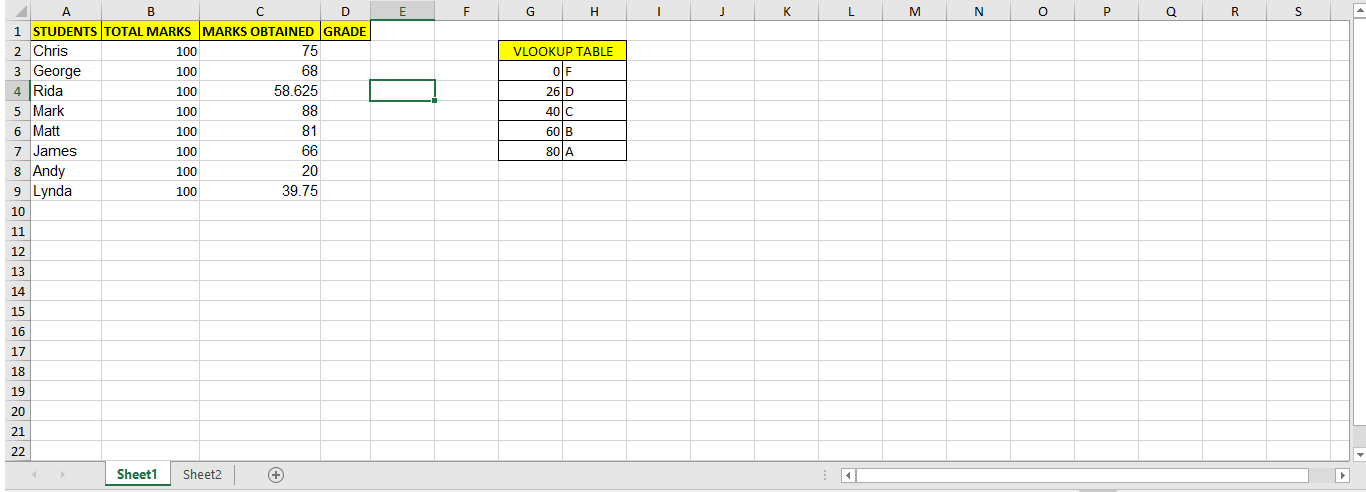
This screenshot shows the names of students (column A), their total marks (column B) and marks obtained (column C). The grade column D has to be filled for which a criterion has been given, i.e.:
The grade in the course is “F” if the total is 25 or less. The grade is “D” if the total is above 25 and less than 40. The grade is “C” if the total is 40 or above but less than 60. The grade is “B” if the total is 60 or above but less than 80; otherwise, the grade is “A.”
Therefore for that purpose, a VLOOKUP table has been created in cells G2:H7 to be filled in column D. Now we will apply the formula in D2 that will be: =VLOOKUP(C2,G$3:H$7, 2)
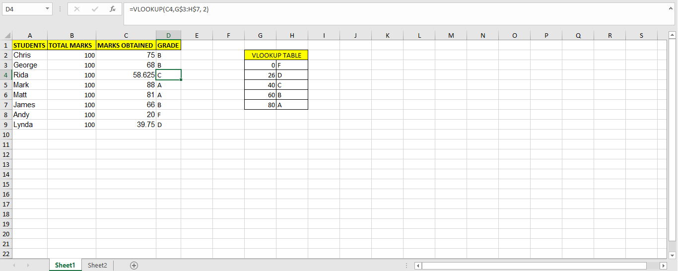
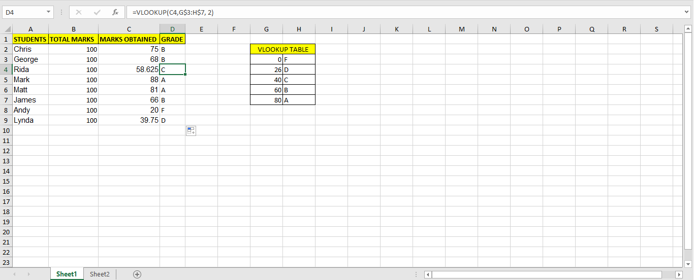
Then drag it down till the last row. This will show us these results:
VLOOKUP Formula Is Copied To Other Column Without Absolute Reference
When we take a look at the above example and the formula we see a “$” sign. This stands for absolute reference. An absolute reference is labeled in a formula by the addition of a dollar sign ($). It is mentioned in the column reference, the row reference, or both. In the example. We have made the lookup table an absolute reference in our formula. The main function of this absolute reference is to hold the value of row number and column name so that the values from the lookup table doesn’t change in the results.
Now as an example, let’s make changes in the formula by removing the absolute reference sign and seeing the results. The formula we used previously in D2 was: =VLOOKUP(C2,G$3:H$7, 2)
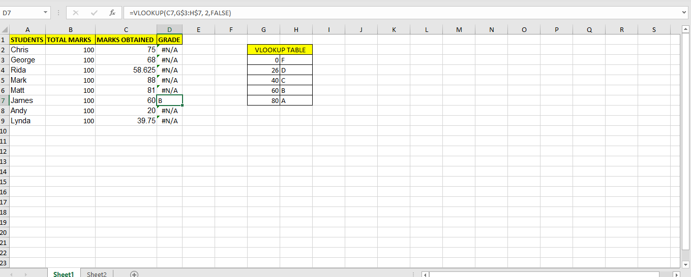
After removing the reference part, we will be left with: =VLOOKUP(C2,G3:H7, 2). Now when we drag this formula across column D, it will give us the following results:
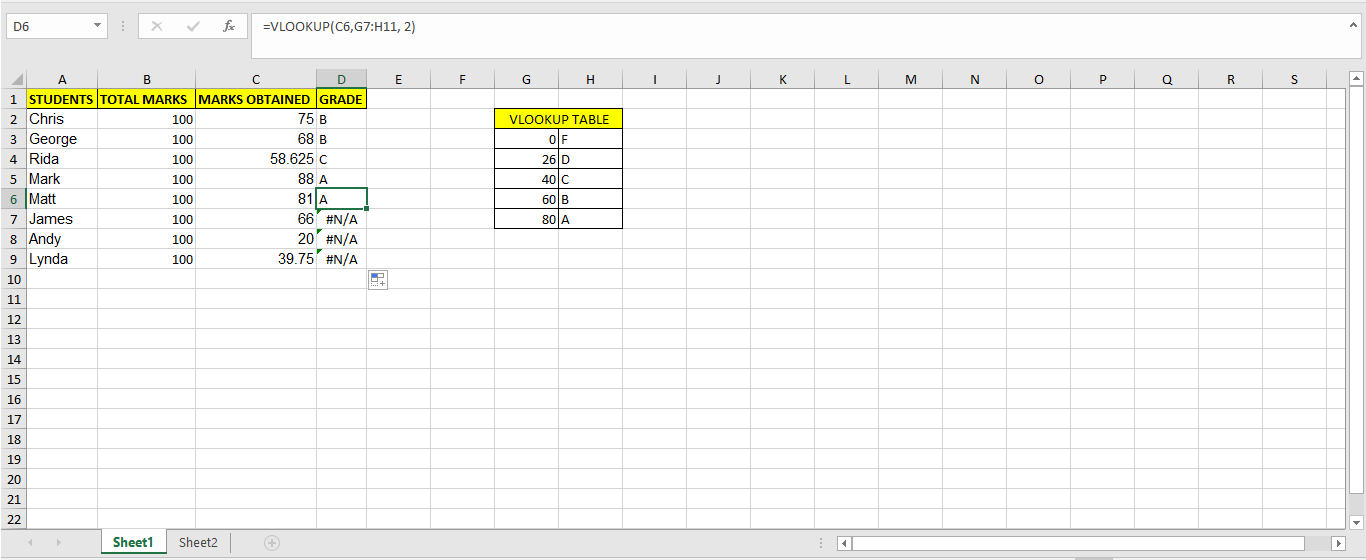
#N/A shows that an error has occurred and the formula was unable to find the grades corresponding to those marks. The reason behind this was that when we dragged the formula, =VLOOKUP(C2,G3:H7, 2), it’s lookup table range G3:H7 was incremented as the formula was dragged which was like this:
=VLOOKUP(C2,G3:H7, 2)

=VLOOKUP(C3,G4:H8, 2)

=VLOOKUP(C4,G5:H9, 2)

=VLOOKUP(C5,G6:H10, 2)

=VLOOKUP(C6,G7:H11, 2)

=VLOOKUP(C7,G8:H12, 2)

=VLOOKUP(C8,G9:H13, 2)

=VLOOKUP(C9,G10:H14, 2)
So this shows that the values of G and H went across the lookup table. The values were supposed to be matched from the table G3:H7 but due to not locking up this table by absolute reference, the lookup table range went till G10:H14 after dragging and it gave an error because nothing exists in G10:H14.
Use VLOOKUP with wrong TRUE/FALSE option
The VLOOKUP function syntax is as follows:
=VLOOKUP (value, table, col_index, [range_lookup])
Where,
value – The value to look for in the first column of a table.
table – The table from which to retrieve a value.
col_index – The column in the table from which to retrieve a value.
range_lookup – [optional] TRUE = approximate match (default). FALSE = exact match.
Now the range_lookup value is optional but very important to be placed in the function. By default “TRUE” is set for this formula even if we don’t write anything. TRUE stands for an appropriate match like it happens when finding a value from a range, while FALSE stands for the exact match.
Let’s take the student grade example in which we wanted to insert grades from a lookup table which defined a specific range.
Now by default if we didn’t enter any range_lookup value, the results were an approximate match as follows:
When we added FALSE in the range_lookup section, we got the following results:
As in this question, we have defined a range, so FALSE is picking the exact value from C columns to be matched with the lookup table. Unfortunately, only one value exists which has an exact match with the lookup table.
Therefore, in some examples entering FALSE is valid but when it comes to having questions which involve picking a value from a defined range, then we can’t use FALSE, it will give us an error.
VLOOKUP on number formatted as text
Another very common problem faced by the user when using the VLOOKUP formula is the mismatch between number and text.
The formula won’t recognize the difference between them. For example:
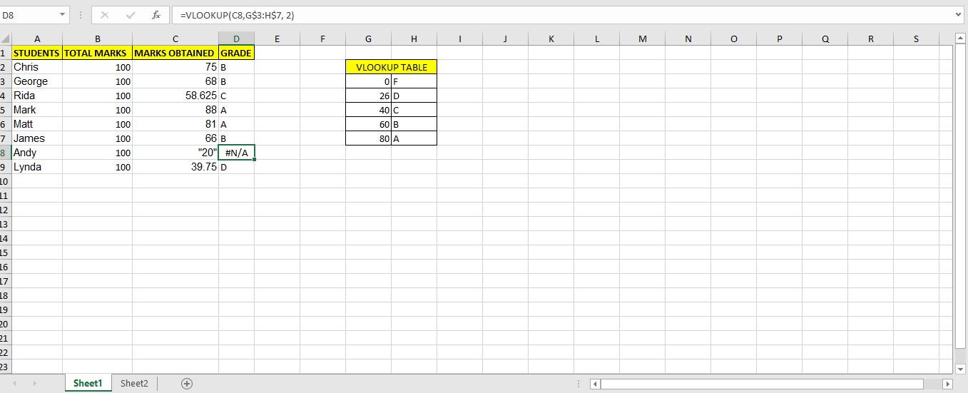
As we see that 20 in C8 is text and therefore it is not picked up by the formula. To convert a text to number, perform the following steps to get rid of the error:
- Select all the entries that you want to ensure are considered TEXT by EXCEL.
- Next, click on the DATA tab and then Text_to_columns.
- In column_data_format, select the option Delimited, and click FINISH.
You will see that the error is removed and it will consider 20 as a number now.
Lookup_value is not on the first column
One VLOOKUP common mistake is that it can only look for values on the most-left column in the table array. If your lookup value is not in the first column of the array, you will see the #N/A error. Let’s have a look at the screenshot below:
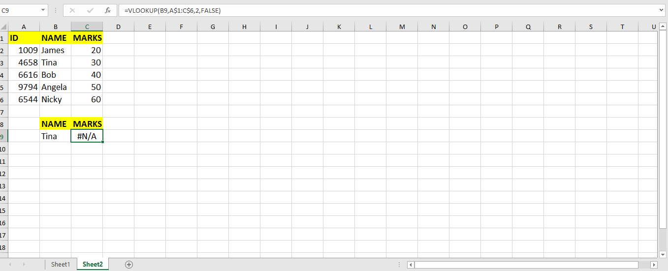
If we look at it, the VLOOKUP formula is returning a #N/A error. The reason behind it is that the lookup value, i.e., NAME: Tina is not in the first column of the lookup table, i.e., A1:C6. If the lookup value is not in the first column of the lookup table then the VLOOKUP formula work.
VLOOKUP Limitations
To use the VLOOKUP function, we must ensure that the data is trimmed and extra spaces are removed from the text.
To do this first, we have to use the “TRIM” function on the lookup value. We must also make sure that the values that are supposed to be returned by the Vlookup but are not returned check if there are any extra characters, spelling mistakes, etc.
VLOOKUP does not handle two or more criteria. Therefore we can’t use it if we want multiple criteria to be defined in our formula.
If you have difficulty using VLOOKUP and want to save hours of reading and researching, you can ask a question to our expert by clicking on this link. You will be connected to a qualified Excel expert in a few seconds, and they will solve your problem on the spot in a live, 1:1 chat session. The first question is free.
Are you still looking for help with the VLOOKUP function? View our comprehensive round-up of VLOOKUP function tutorials here.


Leave a Comment