How to Apply Conditional Format Based on VLOOKUP

Conditional formatting is a great tool to help visualize data on a spreadsheet. It can quickly highlight important information. Conditional formatting comes with many presets that you can apply to highlight your data. However, you can also add your own logic to conditional formatting. 

VLOOKUP is a lookup and reference function to find matches in a table or range by “row.” In this tutorial, we will see how to apply conditional formatting to cells based on the VLOOKUP formula. We will also look at how to copy conditional formats to other cells.

Apply a conditional format based on VLOOKUP

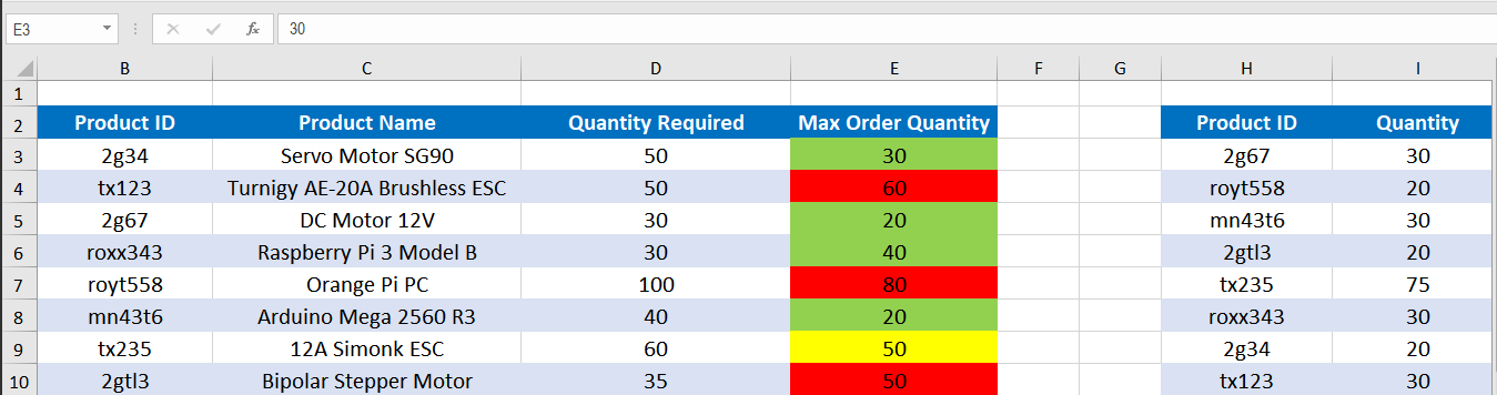
You will work with the Techcom Spares shop inventory and apply conditional formatting based on VLOOKUP. A small part of the data has been represented in cells A1:I10.

Example of using VLOOKUP for conditional formatting

To highlight the products for which the quantity left in stock is currently less than the quantity required:

1. Select cells C3:C10 by dragging from C3 to C10.
2. Click Home > Conditional Formatting > Add New Rule.
3. In the New Formatting Rule dialog box, click Use a formula to determine which cells to format.
4. Under Format values where this formula is true, type the formula: “=VLOOKUP(B3,$H$3:$I$10,2,FALSE) < D3”

5. Click Format.
6. In the Color box, select Red.
7. Click OK until the dialog boxes are closed.

Multiple conditions for the same range

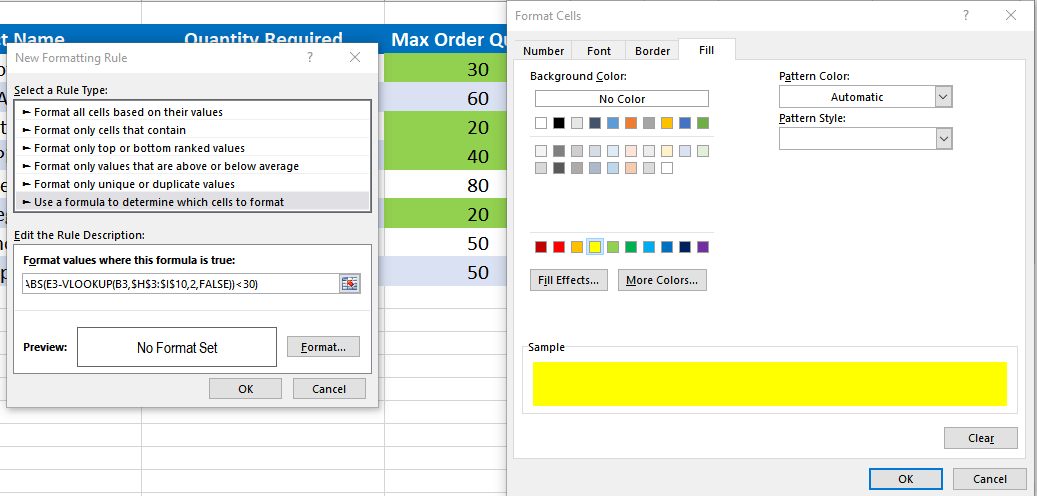
Excel allows us to add multiple formatting rules to the same range. From the previous example, you will highlight the Max Order Quantity into three categories low, medium and high. These will be represented by colors green, yellow and red. To do this,

1. Select cells E3:E10
2. Click Home > Conditional Formatting > Add New Rule.
3. In the New Formatting Rule dialog box, click Use a formula to determine which cells to format. Under Format values where this formula is true, type the formula: “=ABS(E3-VLOOKUP(B3,$H$3:$I$10,2,FALSE))<=10”

4. Click Format.
5. In the Color box, select Green.
6. Click OK until the dialog boxes are closed.
7. Having the same cells selected, repeat steps 2-3, but Under Format values where this formula is true, type the formula:
   “=AND(ABS(E3-VLOOKUP(B3,$H$3:$I$10,2,FALSE))>10,ABS(E3-VLOOKUP(B3,$H$3:$I$10,2,FALSE))<30)”

8. Click Format.
9. In the Color box, select Yellow.
10. Click OK until the dialog boxes are closed.
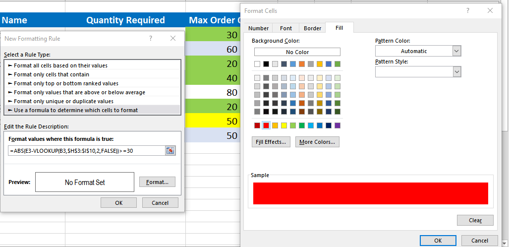
11. For the third color, having the same range selected, repeat steps 2-3. Under Format values where this formula is true, type the formula:
    “=ABS(E3-VLOOKUP(B3,$H$3:$I$10,2,FALSE))>=30”

12. Click Format.
13. In the Color box, select Red.
14. Click OK until the dialog boxes are closed.

Finally, the Max Order Quantity will look like this:

Copy conditional format to another cell

The conditional format can be copied to adjacent cells very easily. If you have adjacent columns that need to be formatted based on the same logic you can use the Format Painter.

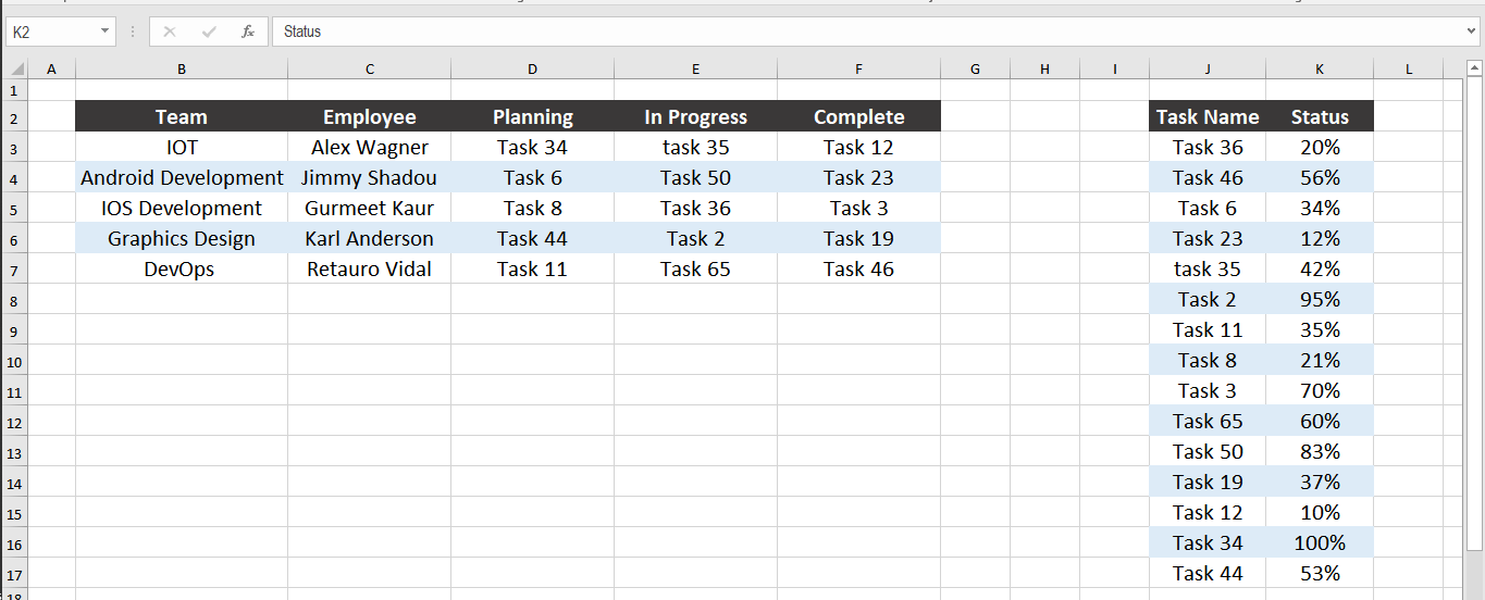
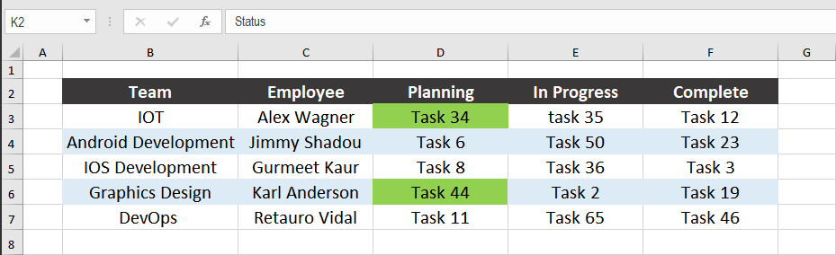
If you want to highlight all the tasks that had progress of 50% or more, you need to:

1. Select cells C3:C7 by dragging by dragging from C3 to C7.
2. Click Home > Conditional Formatting > Add New Rule.
3. In the New Formatting Rule dialog box, click Use a formula to determine which cells to format. Under Format values where this formula is true, type the formula:
   “=VLOOKUP(D3,$J$3:$K$17,2,FALSE) >= 0.5”
4. Click Format.
5. In the Color box, select Green.
6. Click OK until the dialog boxes are closed.

7. To copy the conditional format from column D to E and F, click on cell D3.
8. Click Home > Format Painter.

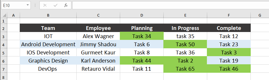
9. To paste the conditional formatting, drag the paintbrush icon to cells E3:F7.
10. Press Esc. anytime to cancel the Format Painter.

    This will copy column D’s format to column E and F.

Conditional Formatting is a fantastic tool in Excel. Shipping with essential presets, you can also add your custom made rules to conditional formats. In this tutorial, we saw such an example with the VLOOKUP function. VLOOKUP is an essential lookup and reference function used to extract values based on a match. Along with VLOOKUP and Conditional Formatting, we can create powerful workarounds like these that help us to visualize our data in a clean and tidy manner.

If you have trouble with using VLOOKUP and conditional formatting and want to save hours of researching, try our Excel Chat live help service. Our experts are available 24/7 and ready to answer any Excel related question on the spot. The first question is free.

Are you still looking for help with the VLOOKUP function? View our comprehensive round-up of VLOOKUP function tutorials here.