Handling an #N/A Error When Using VLOOKUP

1. No match is found:

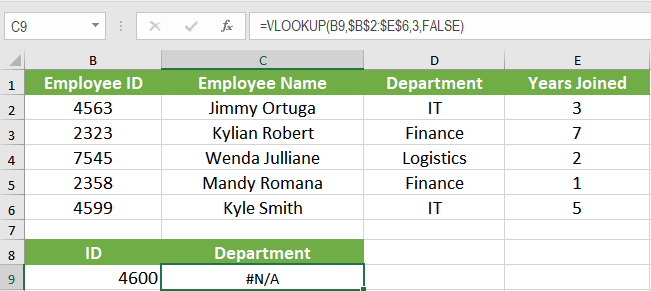
• If range_lookup is set to FALSE and the lookup value does not exist in your table_array, VLOOKUP returns a #N/A. We will use the employee database to demonstrate this. If you wanted to find out the department for ID “4600” using VLOOKUP in cell C9.

  It would return a #N/A as “4600” does not exactly match with any of the entry Employee ID in column A.

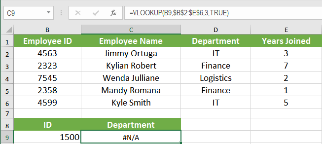
• If range_lookup is set to TRUE and the lookup value is smaller than the smallest value in the table_array, VLOOKUP will return a #N/A error.

  In this example, no values in the range B2:E6 range that is lesser than the lookup_value 1500.

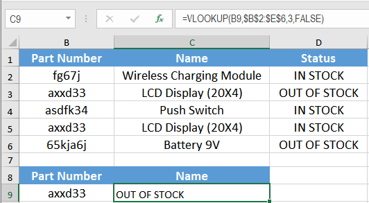
• If range_lookup is set to TRUE and any of the lookup columns are not sorted in ascending order, a #N/A error is returned. In the following example, the range_lookup is set to TRUE, and the lookup column is not sorted in ascending order resulting cell C9 in a #N/A error.

2. Multiple Matches found:

For multiple matches, VLOOKUP pulls over the first match in the table.

Here, the lookup column has multiple matches for the lookup_value. VLOOKUP returns the first match. If we wanted the second match, this wouldn’t be much help.

You can avoid #N/A errors by taking a few precautions. But often, the data is not fully clean and tidy. At these times you need to handle these errors with custom text. In the next section, we will see some functions to handle these errors.

ISERROR() function:

You can use ISERROR() along with IF() to handle VLOOKUP returning #N/A errors. To prevent #N/A error in cell B9,

1. Click cell B9.
2. Click on the formula bar and assign the formula
   “=IF(ISERROR(VLOOKUP(B9,$B$2:$E$6,3,FALSE)),"Employee not found",VLOOKUP(B9,$B$2:$E$6,3,TRUE))”

3. Press Enter.

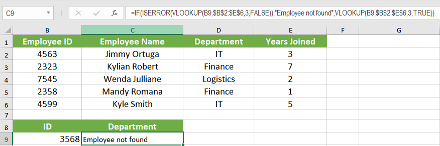
Cell B9 has the value “3568” which is not present in the table_array. This would normally result in a #N/A error. However, the ISERROR() formula nested within the IF() formula handles the #N/A error and outputs our custom message “Employee not found.”

ISNUMBER() function:

The ISNUMBER() function will check if a value is a number. ISNUMBER() will return TRUE when the value is numeric and FALSE when not.

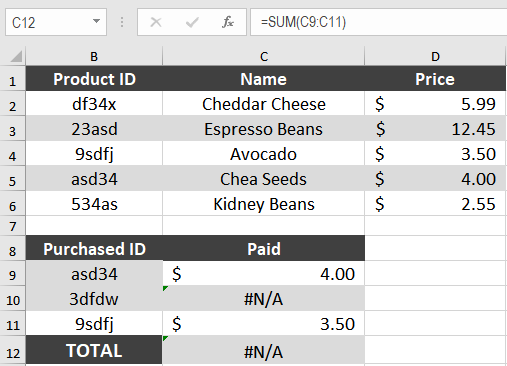
In the following example, you will sum up a grocery bill. The data is on cells B2:B6. On cells B9:B11 we have the purchased items list. The corresponding cells C9, C10, and C11 use the formula to“=VLOOKUP(B9,$B$2:$D$6,3,FALSE)” extract the price. However, cell B10 has product ID 3dfdw which doesn’t have a match in the table_array. As a reason, the corresponding cell C10 is a #N/A. Cell C12 needs to have the total. If you tried to sum C9:C11 you will get a #N/A error as C10 is #N/A.

In order to handle the #N/A error of the prices, you need to:

1. Click on cell C12.
2. On cell C12, assign the formula
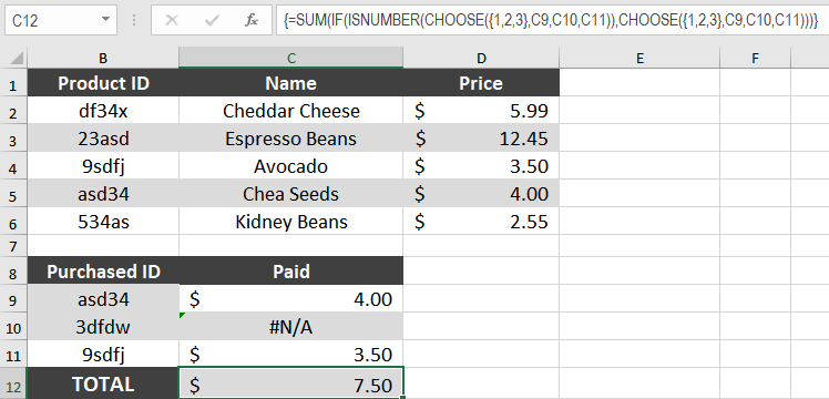
   ” =SUM(IF(ISNUMBER(CHOOSE({1,2,3},C9,C10,C11)),CHOOSE({1,2,3},C9,C10,C11)))”

3. Press Ctrl + Shift + Enter to apply this formula to the cell as it is an array formula. This formula uses the ISNUMBER() and CHOOSE() function nested inside a SUM function. The CHOOSE() function chooses a value from the index which is checked by ISNUMBER() to be a value. Then the resulting numbers are summed and are displayed in cell C12.

VLOOKUP is one of the most effective functions in Excel for lookup and reference. But you need to be careful using it to prevent #N/A errors. Most of these errors can be avoided to some extent. But some errors would remain even after taking all possible measures. For these cases, the existing errors need to be handled. ISERROR() and ISNUMBER() are two such functions used to handle #N/A errors associated with VLOOKUP().

There are many cases in which VLOOKUP may result in errors. Sometimes, the problem is your data set-up. If you want to save hours of researching and frustration, try our Excel Live Chat service! Our Excel experts are available 24/7 to answer any Excel question you have on the spot. The first question is free.

Are you still looking for help with the VLOOKUP function? View our comprehensive round-up of VLOOKUP function tutorials here.