Using VLOOKUP on multiple columns

VLOOKUP is one of the lookup and reference functions in Excel and Google Sheets used to find values in a specified range by “row”. It compares them row-wise until it finds a match. In this tutorial, we will look at how to use VLOOKUP on multiple columns with multiple criteria.

The syntax for VLOOKUP is =VLOOKUP (value, table_array, col_index, [range_lookup]). In its general format, you can use it to look up on one column at a time. However, tweaking the formula allows us to use VLOOKUP to look across multiple columns.

VLOOKUP doesn’t handle multiple columns. In the following example, if we wanted to find the match for both Movie and Showtime column, it wouldn’t be possible with basic VLOOKUP syntax. You can find matches for Movie and Showtime columns individually but to find a match based on both the columns, you would need to modify the VLOOKUP formula.

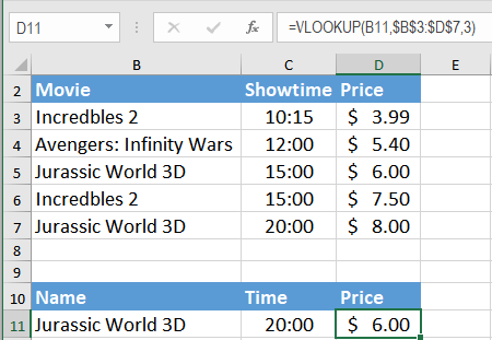
Here, we have a data set in cells B2:D7 that contains the data for ticket prices for different movies at different times. In cell D11 you will return the price for the movie in B11 at the time in C11. B11 has the movie “Jurassic World 3D”. From the data in B2:C7, there are two records for the movie in B11- “Jurassic World 3D”. The ticket for the first show at 15:00 costs $6.00. The second show at 20:00 costs $8.00. In D11 you will look up for the show at 20:00 using the formula “=VLOOKUP(B11,$B$3:$D$7,3,FALSE)”. But this does not return the correct result. To find the accurate result for multiple columns using VLOOKUP you will need to make some modifications to the formula.

Using VLOOKUP on multiple columns

Using the concatenate operator(“&”):

The Concatenate Operator(“&”) helps to use VLOOKUP on multiple columns to satisfy multiple conditions. In the previous example, VLOOKUP failed to return the value for the second instance which fulfilled certain criteria( i.e. the Movie name and Showtime). With the Concatenate Operator, we can specify both the criteria inside the formula which would extract the correct ticket price for our desired instance. However, we have to make sure the range lookup is set to default which is TRUE.

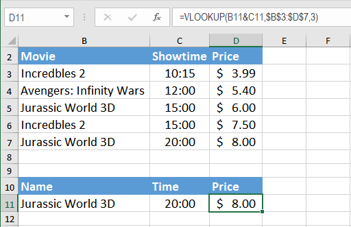
To find the correct ticket price for “Jurassic World 3D” at 20:00:
- Select the cell D11 by clicking on it.
- Insert the formula “=VLOOKUP(B11&C11,$B$3:$D$7,3)”.
- Press Enter to apply the formula to cell D11.
It returns the result $8.00 this time. Looking at the data at cell D7, you can confirm that this is the correct Price for the movie “Jurassic World 3D” at “20:00”.
Using INDEX/MATCH:

You can also use a combination of the functions INDEX() and MATCH() to lookup values based on multiple criteria. INDEX() returns the value of a cell in a table based on the column and row number. MATCH() returns the position of a cell in a row or column. Combining these two functions we can look up a value both horizontally and vertically. The combination of INDEX() and MATCH() overcomes the limitations of VLOOKUP to return value based on multiple criteria.

To solve the problem in the previous example with INDEX()/ MATCH(), you need to follow the following steps:
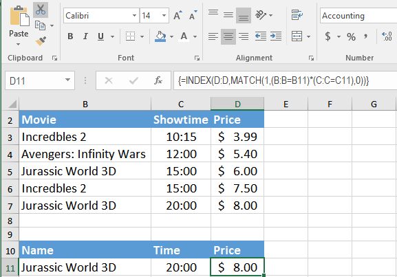
- Select the cell D11 by clicking on it.
- Insert the formula “=INDEX(D:D,MATCH(1,(B:B=B11)*(C:C=C11),0)” in cell D11.
- Press Ctrl + Shift + Enter to insert the formula and turn it into an array formula. Pressing enter will result in a #N/A error. You must press Ctrl + Shift + Enter to make sure the formula returns a valid number.
The INDEX() function returns a value from column D based on the match by the MATCH function with the criteria being B:B = B11 and C:C = C11. The “1” here refers to TRUE as in return the row number where all the criteria are TRUE.

VLOOKUP is a very effective lookup and reference function. Still, it has some limitations when looking for data in multiple columns based on multiple criteria. However, you can overcome these limitations using some modifications to the formula. Using the Concatenate Operator(“&”) or using the combination of INDEX() and MATCH() functions let you extract values from multiple columns.

VLOOKUP based on multiple criteria isn’t applicable. However, sometimes, the problem is your data set-up. If you want to save hours of researching and frustration, try our Excel Live Chat service! Our Excel experts are available 24/7 to answer any Excel question you have on the spot. The first question is free.