

Use VLOOKUP across multiple worksheets
If you want to use VLOOKUP across several worksheets in Excel, you can accomplish this by using the Consolidate feature as well as certain features of the VLOOKUP function itself.
Use Consolidate in Excel with VLOOKUP
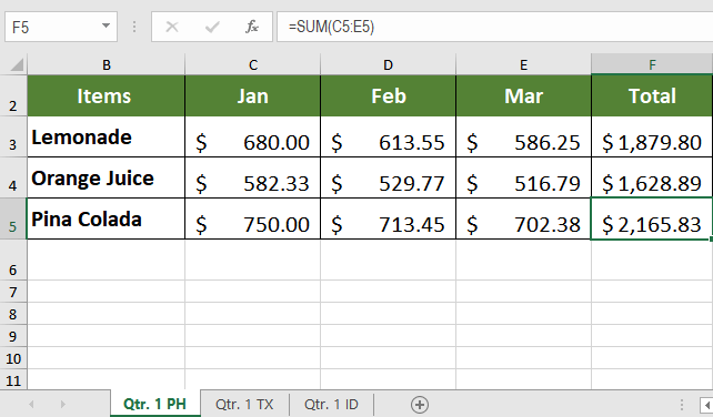
=VLOOKUP(value, table_array,col_index,[range _lookup]).In the following example, we have the sales record of beverages in three different states for the 1st quarter of the year 2018. The workbook contains three sheets of data for sales during the 1st quarter of the year. There are three items: Lemonade, Orange Juice, and Pina Colada. The data contains the sale records for these items during the months January, February, and March. It represents the sales for three states, PH, TX and ID in the same cells B2:F5 for all three worksheets.

If you want to calculate the percent of individual items for any three months of the 1st quarter, you would need to extract the values with VLOOKUP and sum them. But VLOOKUP won’t work here as the sales records are laid out over multiple worksheets.
In this tutorial, we will show you how to use VLOOKUP when the data for table_array is spread over multiple sheets. You will find the percentage of total sales for Orange Juice sales during the month February.
Using VLOOKUP with reference data on multiple sheets
To use VLOOKUP with referenced data on multiple sheets, you will first consolidate the data on a master sheet. Then on the master sheet, a VLOOKUP formula will help to perform the correct calculation. For this to work you would need to follow the steps below:
- Create a new worksheet named “Qtr. 1 Overall” using the “+” icon on the bottom.
- Click on the cell where you want the consolidated data to begin. For consistency with the previous cells, you want this cell to be B2. Select B2 by clicking on it. Now, click Data > Consolidate.
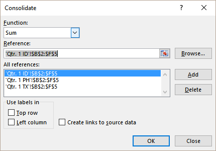
- In the Function box, select the function SUM. In the reference box, first click on the “Qtr. 1 PH” sheet and select cells
B2:F5dragging them with your mouse. Click Add. Click on the “Qtr. 1 TX” sheet. At this point, Excel will automatically have the cellsB2:F5selected. If not, select cellsB2:F5and click Add. Repeat the same process for sheet “Qtr. 1 ID”.![]()
- Click the “Top Row” and “Left Column” checkboxes. If you want the consolidated data to be updated automatically every time the sales sheets updates, click on the “Create links to source data” box.
- Click OK.
![]()

Excel will fill up the newly created worksheet with the sum of all items for the corresponding months. Now, you will make two more changes to the sheet. To add the changes perform the following steps:
- In cells B9 and C9 add the headers “Item Name” and “Month”. These will be the values returned by VLOOKUP. Add the header “Total” in cell D9. This would be the total calculated by consolidation and returned by VLOOKUP.
- In cells B10 and C10, add the name and month “Orange Juice” and “Feb.” On cell D10 insert the formula
“=VLOOKUP(B10,$B$3:$F$5,2,FALSE)/VLOOKUP(B10,$B$3:$F$5,5)“ - Select cell D10, format it as “percentage.” To do this click home > % (On the Number section in the middle).
![]()
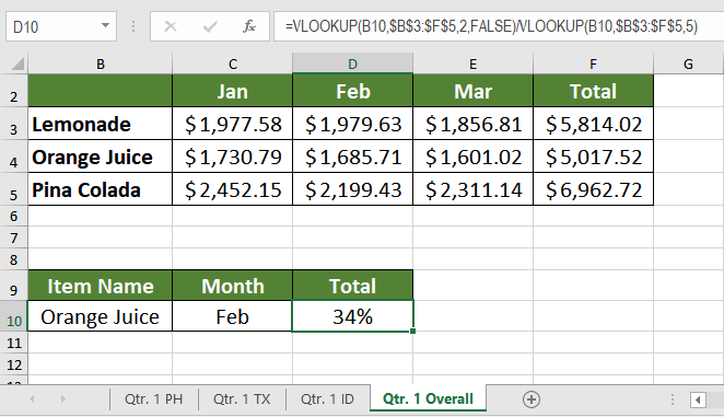
This will return 34% as the percent of total sales for “Orange Juice” for the month of February over the three states.
If you have trouble with using VLOOKUP and want to save hours of researching, try our Excel Chat live help service. Our experts are available 24/7 and ready to answer any Excel related question on the spot. The first question is free.
Are you still looking for help with the VLOOKUP function? View our comprehensive round-up of VLOOKUP function tutorials here.


Leave a Comment